Probability of failure
In CNAIM, the probability of failure (PoF) is modelled as the first three terms of a Taylor Series expansion of an exponential function.
\(\begin{align*} PoF =& K \cdot e^{(C \cdot H)} \\=& K \cdot \sum_{n=1}^\infty \frac{(C \cdot H)^n}{n!} \\\approx& K \cdot \left[1 + (C \cdot H) + \frac{(C \cdot H)^2}{2!} + \frac{(C \cdot H)^3}{3!}\right] \end{align*}\)
where
\(K\) scales the PoF to a failure rate that matches observed fault statistics
\(C\) describes the shape of the PoF curve
\(H\) is the health score based on observed and measured explanatory variables
The definition of a functional failure can be divided into three classes of failure modes:
- Incipient - minor failure
- Degraded - significant failure
- Catastrophic - total failure
Example for a 6.6/11 kV transformer
Assuming a transformer:
- has a utilization of 55%
- is placed indoors
- is sited at an altitude of 75m
- has 20km to the coast
- is sited in an area with a corrosion category index of 2
- is 25 years old
- has a low partial discharge
- has an oil acidity of 0.1mgKOH/g
- has a normal temperature reading
- is in good observed condition
- has a default reliability factor of 1
Then we can call the function as follows:
pof <- pof_transformer_11_20kv(hv_transformer_type = "6.6/11kV Transformer (GM)",
                               utilisation_pct = 55,
                               placement = "Indoor",
                               altitude_m = 75,
                               distance_from_coast_km = 20,
                               corrosion_category_index = 2,
                               age = 25,
                               partial_discharge = "Low",
                               oil_acidity = 0.1,
                               temperature_reading = "Normal",
                               observed_condition = "Good",
                               reliability_factor = "Default")
sprintf("The probability of failure is %.2f%% per year", 100*pof)
[1] "The probability of failure is 0.01% per year"The only mandatory input variablea are transformer type and age; the rest have defaults, so you can call the function like:
pof <- pof_transformer_11_20kv(hv_transformer_type = "6.6/11kV Transformer (GM)",
                               age = 55)
sprintf("The probability of failure is %.2f%% per year", 100*pof)
[1] "The probability of failure is 0.03% per year"It’s also possible to calculate the future probability of failure for a transformer as follows:
library(ggplot2)
library(plotly)
pof <- pof_future_transformer_11_20kv(
  hv_transformer_type = "6.6/11kV Transformer (GM)",
  age = 1,
  simulation_end_year = 80)
ggplot(pof,aes(x=age,y=100*PoF)) +
  geom_line() +
  xlab("Age") +
  ylab("Probability of failure (% per year)")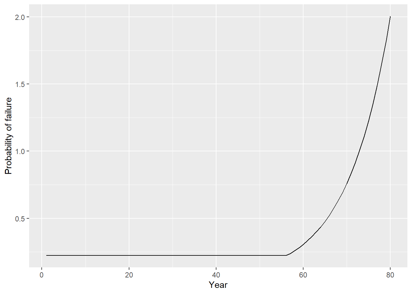
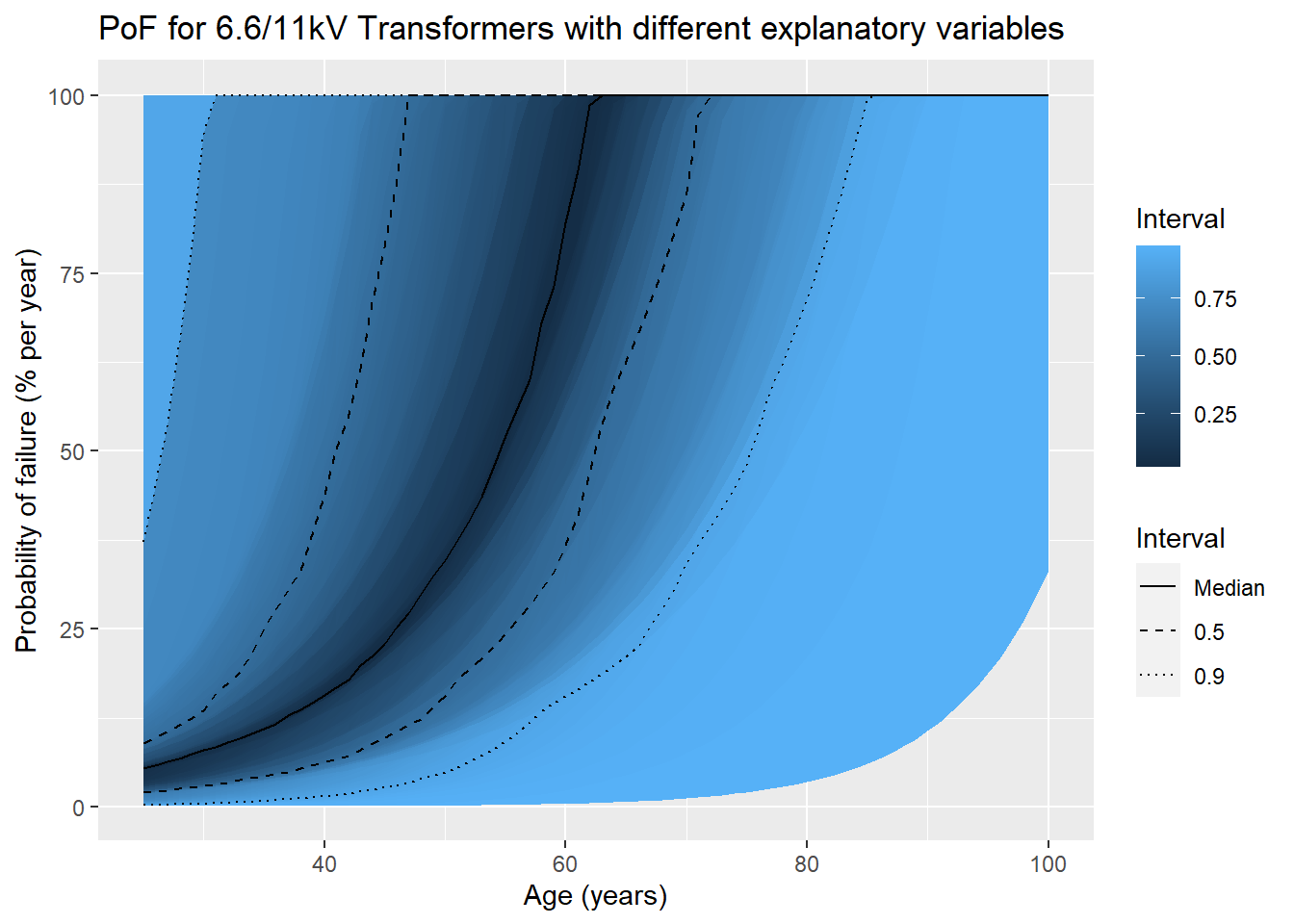
Monte Carlo simulations are able to simulate what happens when all possible inputs are sampled from. The resulting distribution of probabilities is not realistic, since most utilities keep their assets in good condition, but it shows the full range of possible outcomes that the CNAIM PoF model is capable of generating. For 10,000 transformers, we see the following distribution:
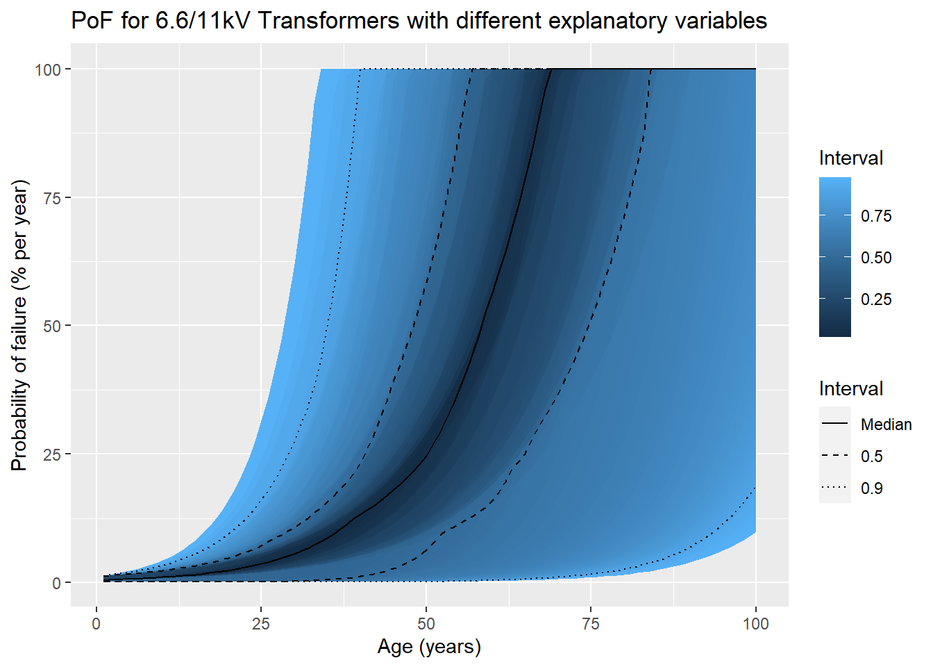
The black line is the median probability of failure and reaches 100% at 69 years. This does not mean that 50% of transformers will have failed at 69 years’ old; the average age is much younger because the probabilities must be multiplied together, year-for-year, assuming independent and identically distributed (i.i.d.) variables. Pulling lifetime estimates in the opposite direction is a strong survivor bias in CNAIM, which means that transformers that have survived e.g. the first 25 years will have a much longer lifetime. If the start year is set to 25, the bias is clearly visible: